

Spread-Spectrum-Modulation
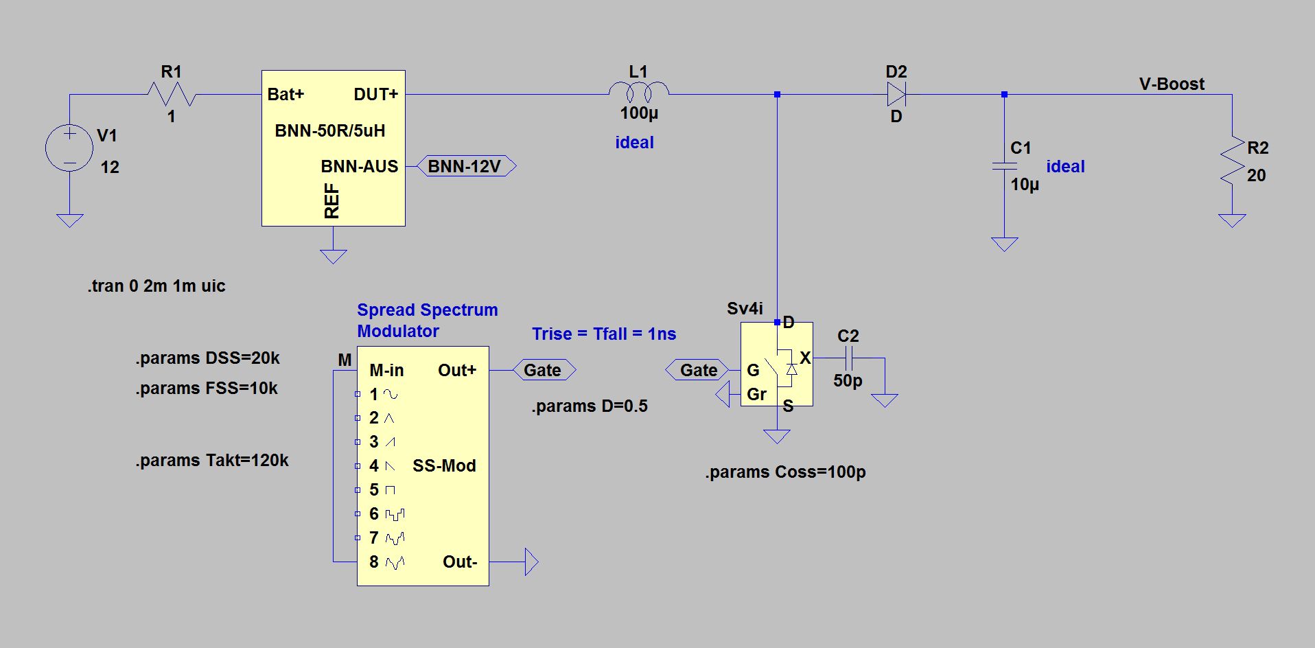
Booster with Spread-Spectrum-Modulation
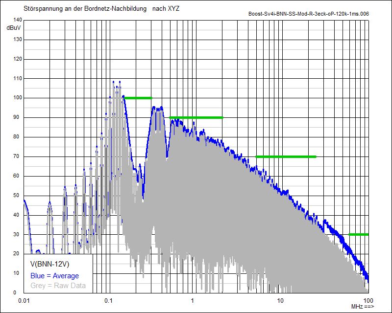
In the following diagrams, the effect of the measuring time on the course of the spectrum is shown in comparison for a random modulation (super-soft) and a triangular modulation. The measuring time is to be seen as the time window for FFT computation. This is somewhat analogous to the measuring time of a detector circuit inside an EMI-receiver.
A priori, one would guess more likely a significant influence of the measuring time for the random modulation - in contrast to a periodically repeating time function (such as the triangular modulation), the stochastic random function has exactly no predictable repetition. The random function corresponds the more to an ideal random distribution, the longer the observation period (the measurement window) lasts.
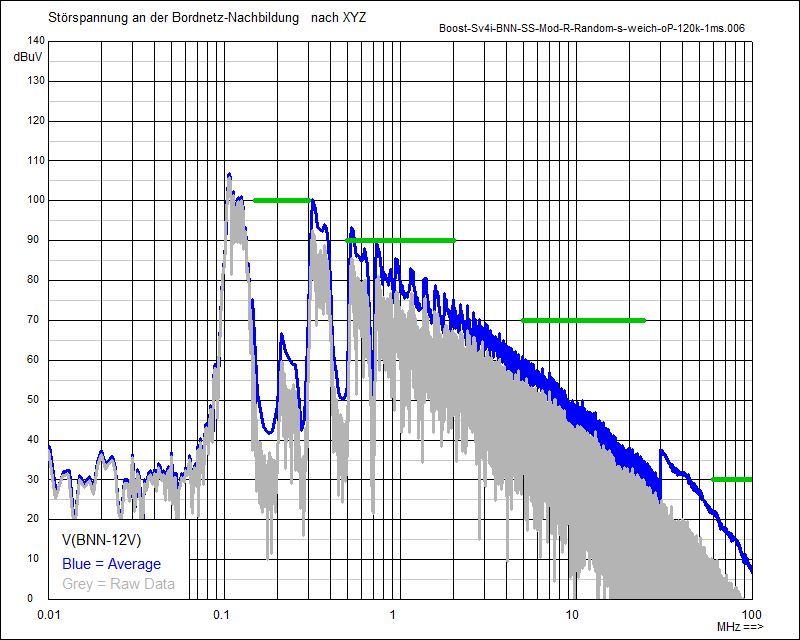
Random Modulation (super-soft) Measuring Time: 1 ms
Triangular Modulation Measuring Time: 1 ms
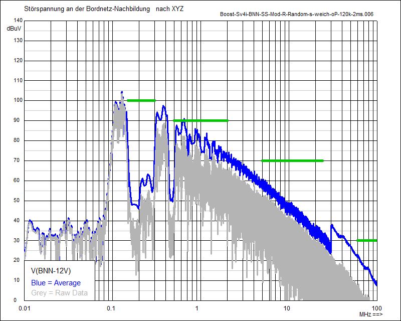
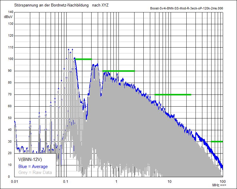
Random Modulation (super-soft) Measuring Time: 2 ms
Triangular Modulation Measuring Time: 2 ms
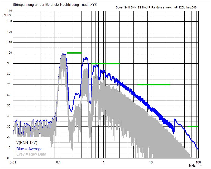
Random Modulation (super-soft) Measuring Time: 4 ms
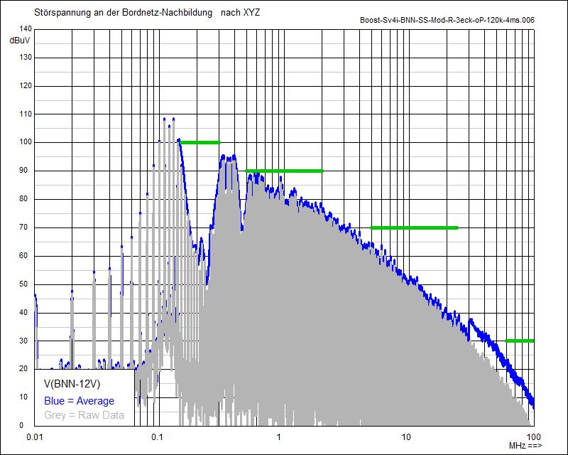
Triangular Modulation Measuring Time: 4 ms
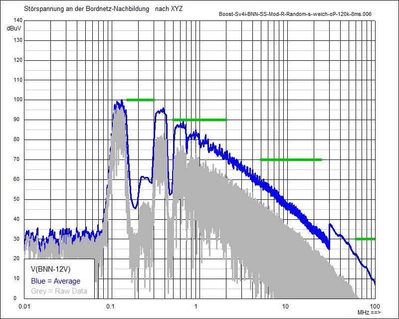
Random Modulation (super-soft) Measuring Time: 8 ms
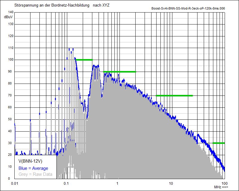
Triangular Modulation Measuring Time: 8 ms
In fact, in random modulation, the effect of the measuring time is clearly visible:
As the measuring time increases, the "spikes" in the course of the curve more and more balance out. It also stands out that the unweighted
spectral lines (the gray areas, raw data) are getting lower in level above 150 kHz. By contrast, the weighted curves (blue, average) largely retain their levels.
The Triangular Modulation is quite different here: the spectral response is almost invariant with respect to the measuring time.
© Ingenieurbüro Lindenberger 8447